Modeling with promor

Introduction

This tutorial shows you how you can use promor to build predictive models using top differentially expressed proteins.

We recommend that you first go through the simple working example provided in Introduction to promor to get acquainted with promor’s functionality.

vignette("intro_to_promor")

A tutorial for proteomics data without technical replicates is provided here: promor: No technical replicates

A tutorial for proteomics data with technical replicates is provided here: promor: Technical replicates

Data

For this tutorial we will be using a previously published data set from Suvarna et al. (2021). In this study, authors used differentially expressed proteins between 33 severe and 18 non-severe COVID patients to build models to predict COVID severity. Here, we are using a subset of that data set (18 severe and 18 non-severe COVID patients).

To build the fit_df and the norm_df objects provided with the pacakge and used in this tutorial, the following analytical steps were conducted:


#Create a raw_df object with default settings
covid_raw <- create_df(
  prot_groups = "https://raw.githubusercontent.com/caranathunge/promor_example_data/main/pg3.txt",
  exp_design = "https://raw.githubusercontent.com/caranathunge/promor_example_data/main/ed3.txt",
)

#Filter out proteins with fewer than 66% valid values in either group
covid_filt <- filterbygroup_na(covid_raw)

#Impute missing data with the minProb method
covid_imp_df <- impute_na(covid_filt)

#Normalize the data with the quantile method
covid_norm_df <- normalize_data(covid_imp_df)

#find DE proteins and make a fit_df object
covid_fit_df <- find_dep(covid_norm_df)

Workflow

promor for modeling flowchart by caranathunge Figure 1. A schematic diagram showing the suggested promor workflow for building predictive models with protein candidates

You can access the help pages for functions shown above and more using ?function_name

Input data

To build predictive models with promor, you need:

A fit_df object produced by running find_dep for differential expression analysis. For this example, we will be using covid_fit_df object provided with the package.
An norm_df object which is a data frame of normalized protein intensities used as input for find_dep. We will be using covid_norm_df object provided with the package.

1. Create a model_df object

Let’s first create a model_df object with the example fit_df and norm_df objects provided with the package.

Notes

pre_process function uses information from the two objects to create a data frame of protein intensities in a suitable format for modeling.

If you run this step with default options, highly correlated proteins (features) will be identified and removed from the data frame.

Alternatively, you can set find_highcorr = FALSE and rem_highcorr = FALSE, but it is not recommended. You can also tweak the corr_cutoff to change the threshold for identifying highly correlated proteins.

Note: if no or few differentially expressed proteins were identified at the given adjusted p-value cutoff, you can choose to relax these criteria to use more proteins in modeling.

See ?pre_process for more information.

# Load promor
library(promor)

# Create a model_df object with the top differentially expressed proteins.
covid_model_df <- pre_process(
  fit_df = covid_fit_df, 
  norm_df = covid_norm_df
)

# Let's take a look at the first few rows of the model_df object
head(covid_model_df)

2. Visualize protein (feature) variation among conditions (classes)

At this stage, we can visualize the feature variation among classes using box plots or density plots.

Notes

Your best proteins (features) for modeling are those that show distinct patterns of variation among conditions.

For example, these proteins may show mostly non-overlapping density distributions.

Feature plots - box plots

# Box plots (default) to visualize feature variation
feature_plot(
  model_df = covid_model_df,
  n_row = 4,
  n_col = 2
)

Feature plots - density plots

# Alternatively, make density plots
feature_plot(
  model_df = covid_model_df,
  type = "density",
  n_row = 4,
  n_col = 2
)

At this stage, if you decide to remove a protein or some proteins from the model_df object, you can do so with rem_feature.

3. Split model_df object into training and test data sets

Next, we will split the model_df object into training and test data sets while maintaining class or condition proportions in each set.

Notes

By default, 80% of the data will be added to the training set while 20% will be added to the test set.

You can change these proportions by setting train_size to a higher or a lower value.

# Create a split_df object by splitting data into training and test data set. Don't forget to fix the random seed for reproducibility.
covid_split_df <- split_data(model_df = covid_model_df, seed = 8314)

Access items in the split_df object.

# You can access the items in the training data set as follows,
covid_split_df$training

# Similarly, access the test data set
covid_split_df$test

4. Train machine learning models on the training data set

We will be using some functions from the caret package to train models on our training data set.

Notes

A list of all the available machine learning algorithms can be found here: http://topepo.github.io/caret/train-models-by-tag.html.

Note that some algorithms may require additional arguments. See caret functions train and trainControl for more details.

The default list of classification-based algorithms provided include:

"svmRadial" - A support vector machine algorithm

"glm"- A generalized linear model algorithm

"rf" - A random forest algorithm

"xgbLinear" - An extreme gradient boosting algorithm

"naive_bayes" - A naive bayes algorithm

For this data-set we chose four algorithms. They were chosen based on their suitability for building models using few features (eight proteins) and samples (35 samples).

# Create a model_list object by training models on the training data set using a custom list of algorithms.Don't forget to fix the random seed for reproducibility.
covid_model_list <- train_models(split_df = covid_split_df, 
                                  algorithm_list = c("svmLinear", "rf", "naive_bayes", "knn"),
                                 seed = 351)

5. Check model performance

We can now check how models built with each algorithm performed on the resamples of the training data set.

Performance plots - box plots

# Box plots (default) to visualize model performance
performance_plot(model_list = covid_model_list)

Performance plots - dot plots

# Make dot plots
performance_plot(
  model_list = covid_model_list,
  type = "dot"
)

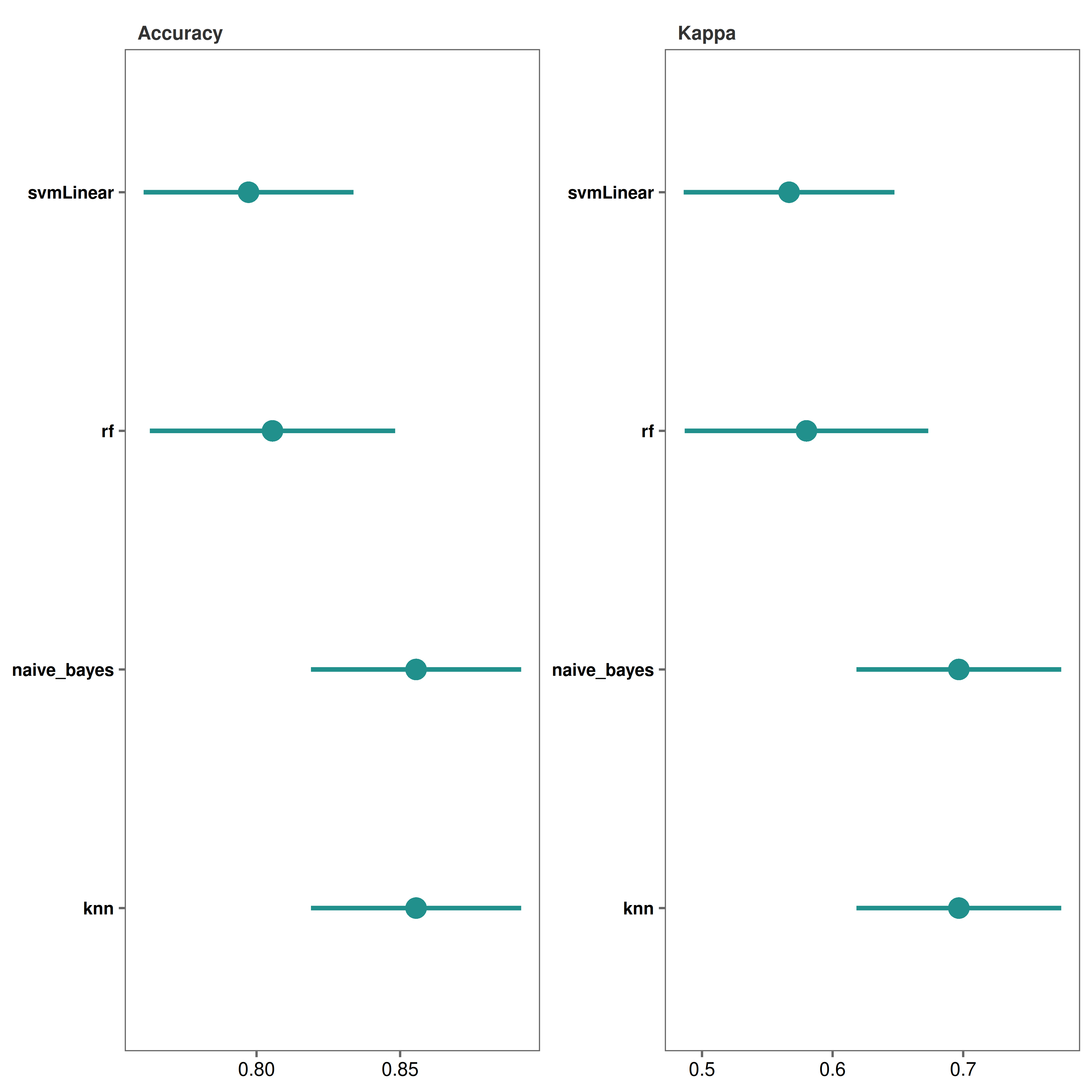
*It looks like both “knn” and “naive_bayes” methods performed fairly well.

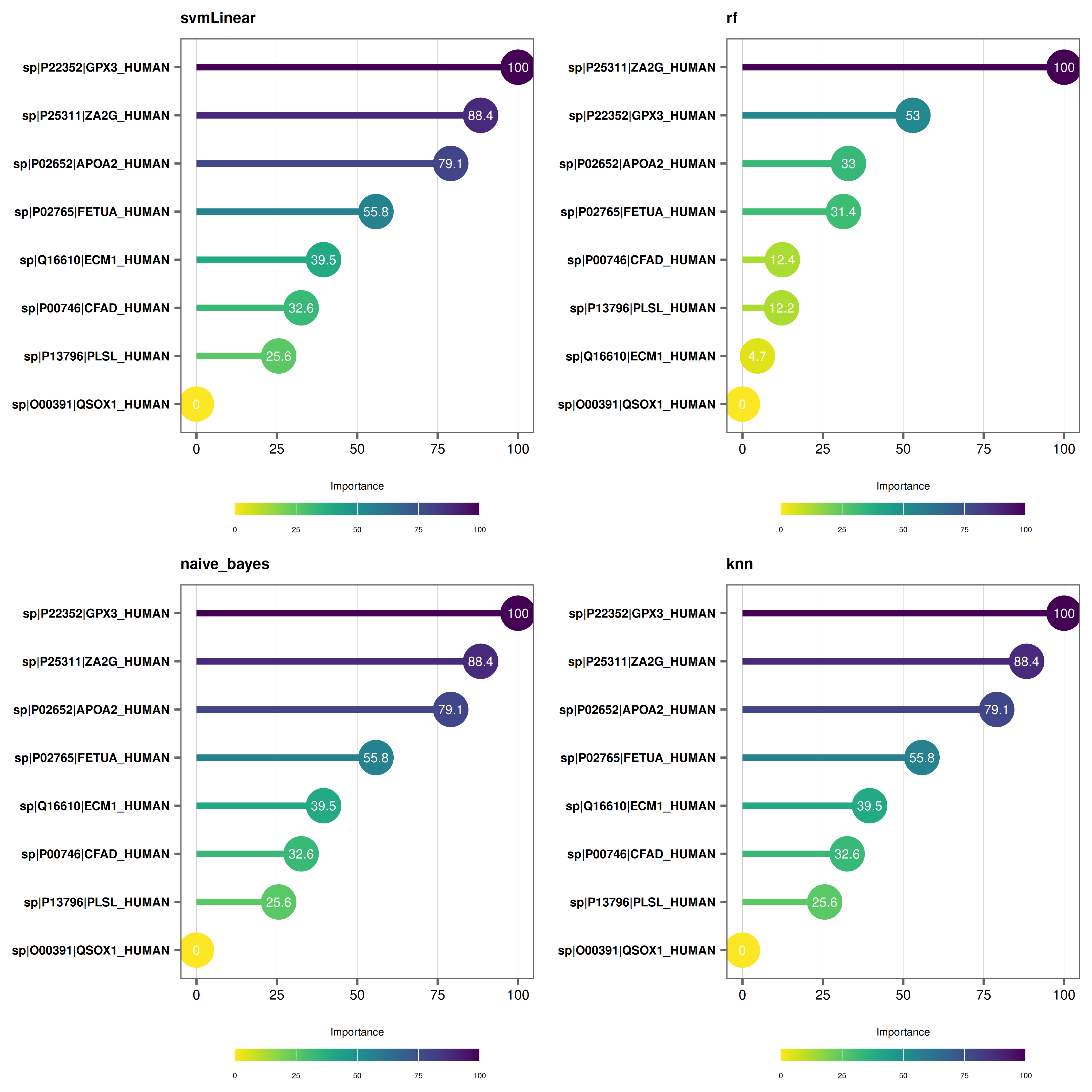
6. Check variable importance

We can check which proteins out of the 8 are most important in the models.

Variable importance plots - lollipop plots

# Make lollipop plots (default)
varimp_plot(
  model_list = covid_model_list,
  text_size = 7,
  n_row = 2,
  n_col = 2
)

Variable importance plots - bar plots

# Make bar plots
varimp_plot(
  model_list = covid_model_list,
  type = "bar",
  text_size = 7,
  n_row = 2,
  n_col = 2
)

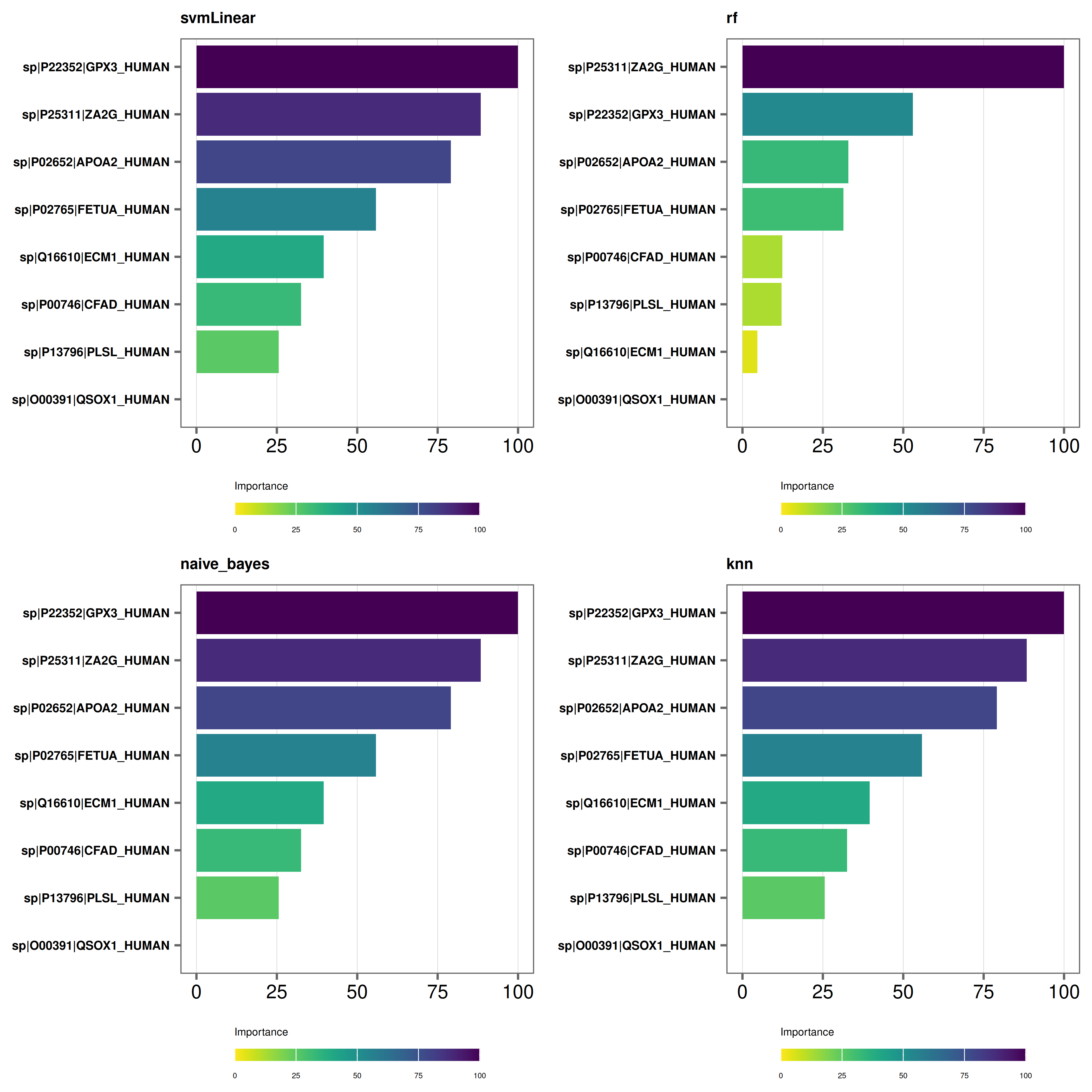
At this stage you can again use rem_feature function to remove proteins with lower importance in the models and repeat steps from Step 3.

7. Test models on the test data set

We are now ready to test our models on never-before-seen data or our test data set.

# First we run the function with type = "prob" to get a probability list
covid_prob_list <- test_models(
  model_list = covid_model_list,
  split_df = covid_split_df,
  type = "prob"
)

Alternatively, you can output a list of predictions and output a confusion matrix for further analysis.

# We run the function with type = "raw" to get a prediction list and output a confusion matrix. You can also provide a file path to save the text file in in your preferred directory. In this example, we are saving our text file in the working directory.
covid_pred_list <- test_models(
  model_list = covid_model_list,
  split_df = covid_split_df,
  type = "raw",
  save_confusionmatrix = TRUE,
  file_path = "."
)

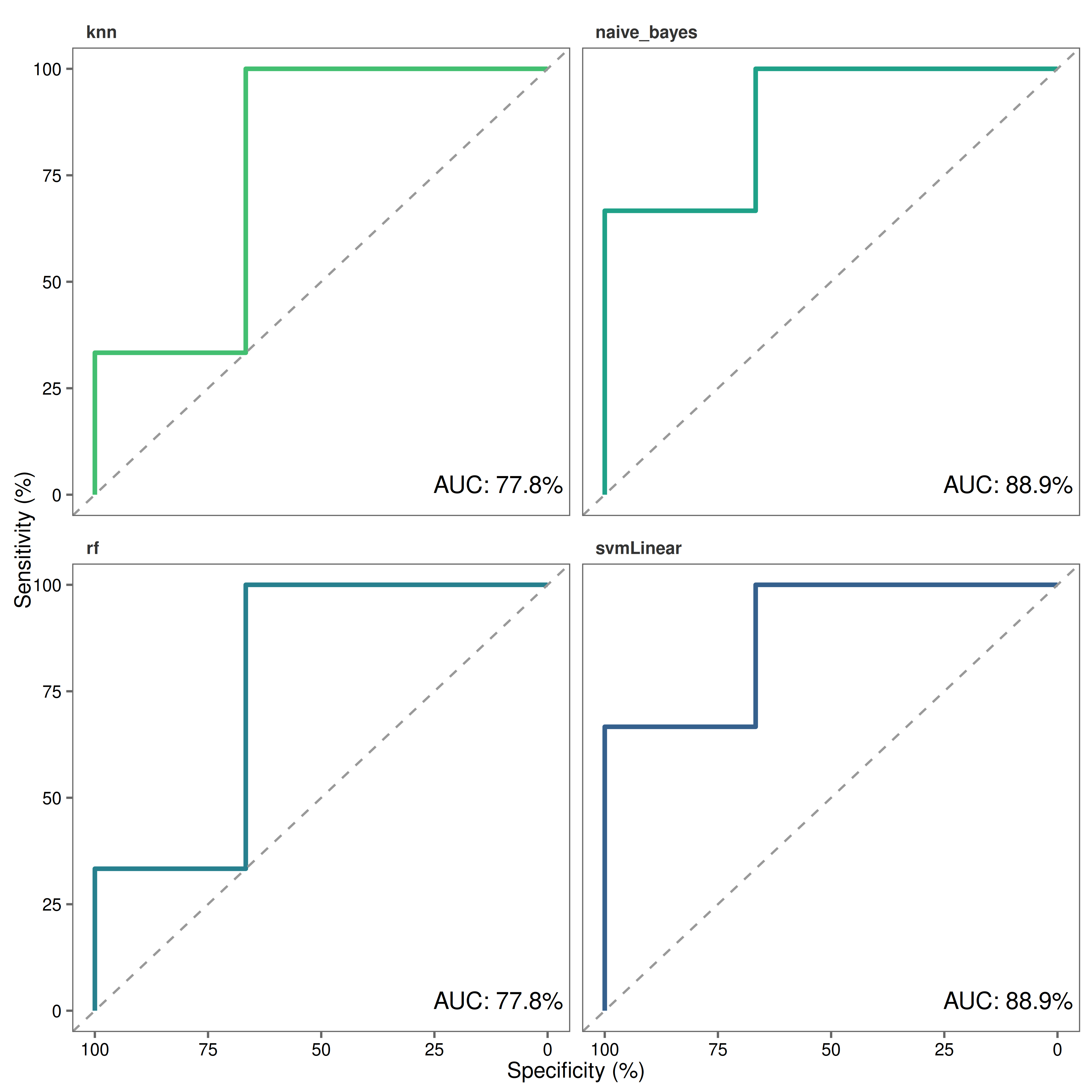
8. Build Receiver Operating Characteristic (ROC) curves

Finally, we can build ROC plots to assess the predictive power of our models.

Notes

roc_plot function requires a probability_list object.

Make sure to set type = "prob" when running test_models to output a probability_list object.

# Make roc curves
roc_plot(
  probability_list = covid_prob_list,
  split_df = covid_split_df
)

Save a copy of the plot in the working directory.

# Make roc curves
roc_plot(
  probability_list = covid_prob_list,
  split_df = covid_split_df,
  save = TRUE,
  file_path = "."
)

Chathurani Ranathunge